How Accurate Are AI Trading Bots? The Limits of Neural-Network Price Forecasting
Over the past three years, rapid progress in artificial intelligence has fuelled a surge of interest in agentic trading: AI agents that do more than analyse markets. They gather information, make decisions and execute trades on their own.
Academic reviews paint a more cautious picture. Many published experiments with LLM-based trading agents do not properly account for transaction costs, out-of-sample testing, survivorship bias or reproducibility (Yao & Zheng, 2026). A 2026 survey of 34 studies found that evaluation methods across the field are inconsistent (AL-Aldaffaie et al., 2026). Regulators share the concern: FINRA and the Bank of England point to the autonomy of these systems, the adequacy of controls and auditability, and the risk that many AI systems will converge on similar behaviour.
Far less attention goes to a more basic question: how accurate are neural-network forecasts of market prices in the first place? Every AI system that makes market decisions relies on some kind of price forecast. In some trading bots it is hidden inside the decision pipeline; in others it is a separate component, built with one of many neural-network architectures and assumed to be good enough. Either way, forecast accuracy sets the ceiling for everything that comes after it.
The rapid adoption of agentic trading quietly treats price forecasting as a solved problem. History suggests otherwise: classical mathematical methods of the pre-neural-network era never produced a convincing general solution.
Based on several years of our own research and experiments with neural-network and classical forecasting, and our work with automated trading bots, we take the opposite view. Despite an extensive search of the published literature, we have not found convincing evidence that neural-network forecasts of financial prices are consistently effective.
In this article we look at how accurate these forecasts really are, why they break down, what that means for AI trading bots, and one approach we use to improve them.
Key Takeaways
Neural-network (LSTM) price forecasts look accurate only when price spikes beyond one standard deviation are left out of the error calculation.
Once every candle is counted, forecast error becomes almost equal to normal market volatility.
In our crypto samples, spikes make up roughly 15-20% of observations and dominate forecast error.
Price and volume history often contains no information about the external events that cause these spikes, so their timing cannot be predicted from it.
AI trading bots that rely on such forecasts may have no edge exactly when the largest gains and losses happen.
Normalising data around self-similar (multifractal) structures lets a single model generalise across assets and timeframes.
How Accurate Are Neural-Network Price Forecasts?
The practical accuracy of price forecasts depends far more on the nature of financial markets than on the choice of model. To show this, we use arguments that hold largely regardless of architecture, and take as our example the widely used Long Short-Term Memory (LSTM) network — the same architecture behind Teresius Forecast.
LSTM and other recurrent networks have been applied to financial time series for years, and some studies report clear advantages over classical methods. A well-known example is the work of Fischer & Krauss (2018), which showed strong LSTM results in forecasting US equities.
We do not go into the technical details of building the model here. Methods differ, but the field now has a broadly established methodology, and technical choices change accuracy only somewhat. In most practically important cases, the decisive factor is the set of limits imposed by the statistical properties of financial markets themselves.
Forecast Error vs. Volatility: BTCUSDT and GBPUSD Examples
Figures 1 and 2 show BTCUSDT on the 4-hour timeframe and the GBPUSD Forex pair on the 2-hour timeframe. The candles are actual historical prices. The red lines are neural-network forecasts of the High, Low and Close values for the same candles. Both models were trained on historical High, Low, Close and Volume data with a lookback window of 70 candles.
The key comparison is between two numbers:
Market volatility over the 70-candle window — the standard deviation of each price value from its mean (shown on the charts as Sigma High, Sigma Low and Sigma Close).
Forecast error — the standard deviation of the forecast from the actual value (shown as Sigma Forecast High, Low and Close).
On this basis, the forecasts look convincing. For BTCUSDT, the High forecast error is 242.9 against High volatility of 619.7. For GBPUSD, it is 0.00051 against 0.00100. In both cases the error is less than half of normal market movement.
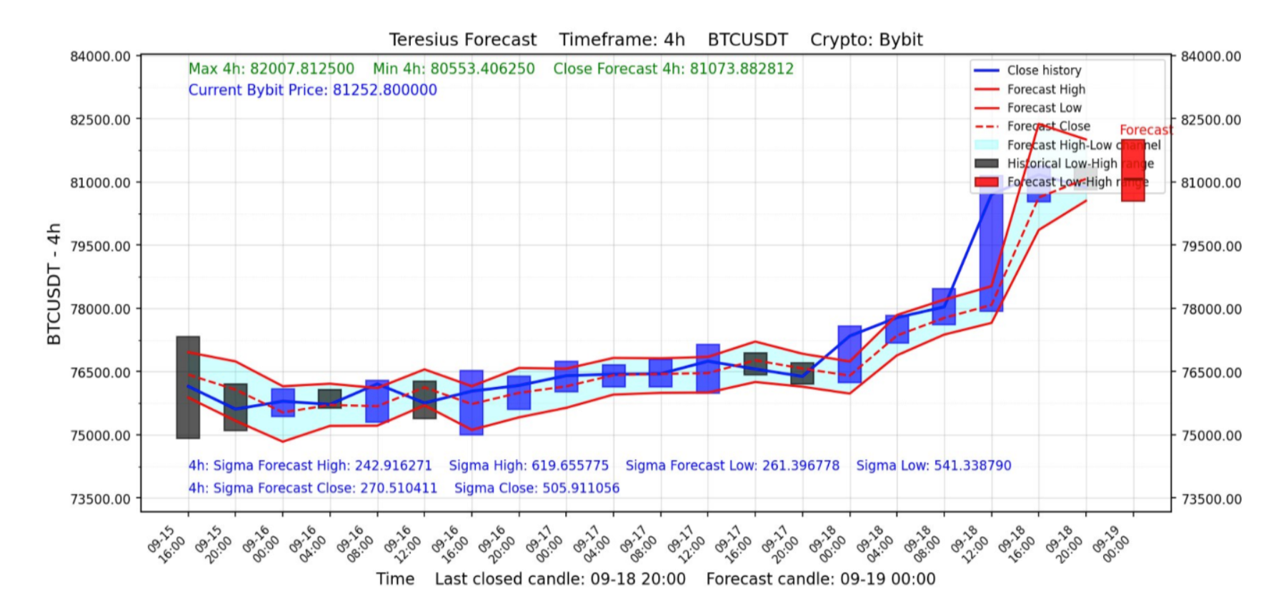
Figure 1. Forecast of BTCUSDT High, Low, and Close values, timeframe = 4h
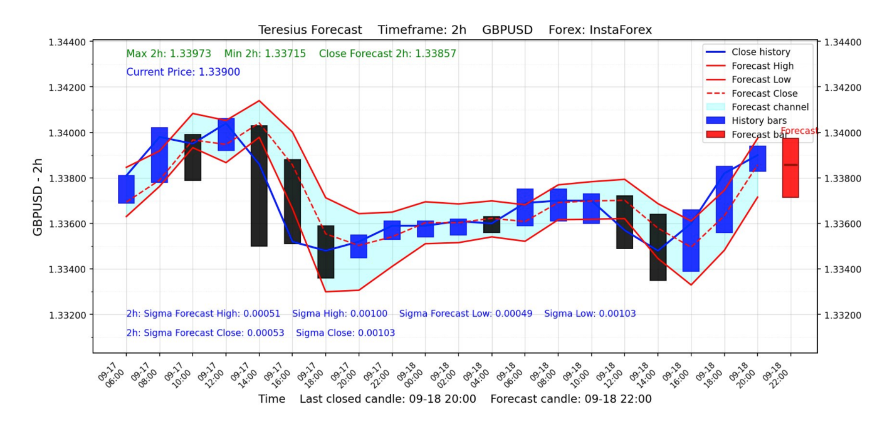
Figure 2. Forecast of GBPUSD High, Low, and Close values, timeframe = 2h
What Happens When Price Spikes Are Included
There is an important detail behind these numbers. The forecast error is not calculated over all 70 candles. It includes only candles where the gap between forecast and actual value is within one standard deviation of volatility. Observations beyond one sigma — the price spikes — are excluded. This filtered figure describes how the model performs in normal market conditions, and it is the SIGMA Forecast value shown on our charts.
When every candle is kept, including the spikes, the forecast error and market volatility become nearly identical. That is a fundamentally different result. In our view, it is not an artefact of a particular modelling approach. It reflects the statistical nature of financial prices.
Why Price Spikes Can't Be Predicted from Price History
Sharp moves are not necessarily random. They can be caused by economic releases, regulatory decisions, news, large-scale liquidations or the actions of major market participants. But a model that sees only historical High, Low, Close and Volume data has no information about a future external event. The timing of such a move cannot be reconstructed from past prices alone.
This is one of the fundamental limits of statistical forecasting. Historical datasets contain many anomalous moves, but their timing may be effectively unpredictable from the data the model has before the event.
It is also well established that returns in financial markets are far from normally distributed. Heavy tails, volatility clustering and extreme price changes are known stylised facts of financial markets (Cont, 2001). So we do not claim that every extreme move is "purely random". The cause may well exist. The point is narrower: the information needed to anticipate the event may simply not be present in the price and volume history the model is trained on.
The Bank of England highlights a related risk for more complex AI models: they may behave unexpectedly in volatility regimes or market conditions that differ materially from their training data. Extreme events and radical uncertainty remain especially difficult.
This is different from non-stationarity in general. Some regular forms of non-stationarity, such as a steady linear trend, can be forecast reasonably well. The problem here is local, irregular and effectively unpredictable market shocks. In our cryptocurrency samples, such spikes account for at least 15–20% of observations across many timeframes. This figure refers to our own samples, not to the market as a whole. Because variance is quadratic, these observations contribute disproportionately to forecast error.
Can this be built into a forecasting model? We know of no generally accepted method that solves the problem directly. Even if one is possible, it is mathematically and statistically non-trivial, and a purely formal treatment is unlikely to be enough.
Our arguments are empirical and conceptual, not a formal mathematical proof. Still, they suggest that many AI trading agents face structural limits when their decisions depend heavily on forecasts built from historical market data alone.
What This Means for AI Trading Bots
A forecast that looks accurate on a chart can still lead to losing trades. The reasons follow directly from the results above.
No edge when it matters most. If forecast error during spikes is as large as the market's own volatility, a bot relying on that forecast is effectively guessing during the very moves that produce the largest gains and losses.
Filtered accuracy overstates real performance. Accuracy measured only in calm conditions says little about how a strategy will survive the 15–20% of candles where most of the risk sits.
Costs eat the remaining margin. Transaction costs, spreads and realistic execution are often missing from published experiments (Yao & Zheng, 2026). Any small advantage in calm markets can disappear once they are included.
Similar models, similar mistakes. When many agents rely on similar models trained on the same price history, they may misjudge the same events at the same time — the correlated-behaviour risk highlighted by the Bank of England.
None of this means forecasts are useless. It means they should be read as a range of likely prices under normal conditions, together with their error and the market's volatility — not as a signal that can be traded blindly.
Can AI Forecast Accuracy Be Improved?
We now turn to a forecasting scheme designed to do two things: identify the parts of price history that are inherently hard to predict, and partly account for another key feature of markets — their constant evolution. Markets rarely repeat earlier patterns exactly, even when similar-looking shapes reappear. In practice, the market often stops behaving the way a model learned from history says it should. Our first goal is to reduce the impact of this poorly predictable evolution.
Multifractals and Market Prices
Traders have noticed visually similar patterns in price charts for more than a century. Mathematically, this behaviour can be described in terms of multifractal, or approximately self-similar, structures. A neural network may learn such structures directly or indirectly during training.
A foundational contribution here is the Multifractal Model of Asset Returns (MMAR) by Mandelbrot, Fisher & Calvet (1997). Later reviews document a large body of research on multifractal properties across many financial markets (Jiang, Xie, Zhou & Sornette, 2019).
This should not be over-interpreted. Multifractality does not mean that markets are made of deterministically repeating shapes, or that future prices can be read off such patterns. The more precise statement is that financial time series can show scale-dependent, statistically self-similar properties. These are the properties Teresius Forecast uses in its multifractal pattern analysis.
Normalising Data to Find Self-Similar Structures
Forecasting performance depends on many aspects of network design and data preparation. In our experience, one of the most important is how the dataset is normalised. Modern training methods can sometimes work without explicit normalisation. We use a specific form of it, designed to expose approximately self-similar structures before training begins.
This normalisation has two goals. It improves the numerical scaling of the data and can speed up training. More importantly, it turns the price history into a set of geometrically comparable fragments, so the network is trained on these structures rather than on raw prices. Any definition of self-similarity based on a mathematical transformation involves some methodological choice.
In a first approximation, the procedure works as follows:
Using a rolling window, extract fragments of historical High, Low, Close and Volume data of length L.
For each variable in each fragment, calculate its arithmetic mean and divide every value by that mean.
Collect the normalised fragments into arrays.
Within each fragment, remove local patterns whose values exceed k × sigma, where sigma is the standard deviation of the normalised fragment and k is a coefficient chosen experimentally.
Bring all fragments to a common length; fragments that become too short are shortened further or dropped.
This differs from conventional normalisation in two ways. It is applied separately to many local fragments rather than once to the whole dataset, and it does not divide by the standard deviation. We chose it because it gave useful results in our experiments with self-similar structures; other methods with the same goal are certainly possible.
The resulting training set mainly describes market fragments in a sideways or flat regime. The network trained on it is the model behind our Telegram bots for cryptocurrency and Forex forecasting.
One Model Across Assets and Timeframes
These experiments produced a result we find noteworthy: the same model, with the same parameters and coefficients, is applied across different cryptocurrency pairs, Forex instruments and timeframes.
For now, we treat this as an experimental observation, not a proven law. But it suggests an interesting hypothesis: an effective financial forecasting model may need, above all, to generalise market structures across instruments rather than memorise the behaviour of any single one. This hypothesis can be tested empirically.
Conclusion
Neural-network price forecasts are useful in normal market conditions, but they are not the solved problem that the rush toward agentic trading assumes. Once price spikes are counted, forecast error approaches the market's own volatility. Because those spikes are driven by events that price history does not contain, no choice of architecture fully removes this limit.
This has a direct consequence for AI trading bots: an accurate-looking forecast is not the same as a profitable strategy. Anyone building or using such systems should ask how accuracy was measured, whether spikes were included, and how the strategy behaves when they occur.
We do not claim to have solved the problem. Our approach — normalising data around self-similar structures and training one model across many assets — is one practical step, and its central hypothesis is open to testing. That is why every Teresius Forecast chart shows past forecasts alongside real prices, together with forecast error and market volatility, so you can judge the results yourself. See how to read a Teresius Forecast chart.
Try Teresius Forecast for free — no registration needed:
FAQ
Can AI trading bots accurately predict crypto prices?
In normal market conditions, neural networks can track price ranges reasonably well. Once sudden price spikes are included, forecast error approaches ordinary market volatility, which limits how reliably a bot can trade on forecasts alone.
Why do price spikes reduce AI forecast accuracy?
Spikes are often caused by news, regulatory decisions or large liquidations. Information about these events is absent from historical price and volume data, so a model trained on that data cannot anticipate their timing.
Is an accurate forecast the same as a profitable trading bot?
No. Accuracy is often measured only in calm conditions, while most risk sits in spikes. Transaction costs and execution can also erase a small forecasting advantage.
What is multifractal analysis in financial markets?
It measures how price patterns repeat in a statistically similar form across different timescales. It does not mean prices follow fixed, repeating shapes.
Does Teresius AI use a separate model for each asset?
No. The same model, with the same parameters, is applied across crypto pairs, Forex instruments and timeframes.
Disclaimer: This article is for research and educational purposes only and is not financial or investment advice. Past forecast performance does not guarantee future results.
References