Ergodicity in Bot Trading: The Hidden Problem of Short Intervals
Hundreds of publications on trading in financial markets appear every day. They cover the widest range of topics: indicators, risk management, machine learning, backtesting, model overfitting, commissions, slippage, and of course the automation of trading.
A substantial portion of these publications is devoted to trading bots. According to open sources, the share of automated and high-frequency trading in a number of segments of financial markets has long been very significant: the Bank of Canada, in an earlier review, noted that HFT accounted for approximately one quarter of the Canadian equity market and more than half of the United States equity market [1]; the SEC and CFTC have likewise examined in detail the growth of automated trading and its influence on market structure [2].
Given the unusually amplified, in our view sometimes excessively amplified, topic of AI's influence on the effectiveness of bot construction, this area finds itself at the centre of attention with particular frequency. We have already offered our view on this question in a previous analytical review [3].
However, most publications on this topic unfortunately share one serious weakness: the absence of concrete material grounded in the actual statistics of real bots in operation. Theory is of course necessary. But no theory can fully fit all the subtleties of trading automation into the specific Procrustean bed of practice.
In this article we examine one of the less-discussed problems of automated trading: the problem of ergodicity and the initial state of a trading bot. We discuss it using a trend-following / momentum bot, more specifically a short-term EMA-slope momentum bot. We emphasise immediately that most of the aspects discussed here apply not only to this specific algorithm. They arise in nearly all bots that make decisions on short trading intervals.
Simulation and Reality: Why Agreement Does Not Come for Free
Suppose you have built a bot to trade on short intervals. The first important point is obvious: such a bot almost certainly has a number of parameters. Sometimes few. Sometimes a great many.
These parameters are usually selected by simulating trading on historical data. And here Einstein's dream of universal equations of the world, equations free of all constants and parameters (including the speed of light), does not hold. In real trading, parameters exist. They have to be selected, validated, re-evaluated, and, what is especially important, correlated against live trading.
Achieving close agreement between simulation results and live trading on an exchange is an extremely difficult task. But it is of primary importance.
Let us consider several aspects that are difficult to reproduce correctly in simulation.
The first is the speed of decision-making in online mode. If a bot does not operate over WebSocket but periodically requests quotes through a REST API, it inevitably accumulates delays, rate limit constraints, and a risk of disagreement with what we subsequently see in the historical candles. Exchanges document such constraints directly: Bybit's API documentation specifies a default rate limit of 600 requests within a five-second window per IP [4], and Poloniex separately recommends the use of WebSocket for real-time data, since its REST API imposes strict access frequency controls [5].
In practice, for accurate simulation, we often descend to the smallest available historical timeframe, often 1m candles. And here lies a trap. Short-timeframe historical data is not always available in the required volume, is not always conveniently downloadable, and the most recent candles may be revised or differ from what the bot saw at the moment of decision. Even the manner in which candles are represented carries weight: historical klines are typically returned as candles of a defined interval, anchored to the candle's open time [6].
Beyond this, several phenomena that arise in real trading are particularly difficult to incorporate into a simulation model: slippage, partial fills, latency, discrepancies between expected and actual execution price, the specifics of contract quantity rounding, commissions, funding payments, stale orders, API failures, and the rest of the reality of trading. Slippage, in the standard definition, is the difference between the expected execution price and the actual price at which the trade occurs [7].
Now suppose that we have achieved a nearly precise algorithmic correspondence between the simulation model and the live bot. Suppose further that commissions, leverage, position sizing, stop-loss, take-profit, and all entry and exit conditions have been reproduced as accurately as possible.
And this is still not the whole picture.
The Bot as a Finite-State Machine With Memory
After simulation, you apply the chosen parameters in real trading. The following question arises: how quickly might these parameters become obsolete as the market evolves?
But a more subtle question lies deeper.
A real bot, in contrast to a "clean" simulation, almost always operates from a particular point in time as a finite-state machine with memory, an initial state, and an execution phase.
It may have:
an open position;
a recently closed position;
a waiting period after a close;
stale TP/SL orders;
a last signal;
a balance already modified by previous trades;
an accumulated state of long and short statistics;
an internal flag permitting or prohibiting entry.
In simulation, these often do not exist. Simulation often starts from scratch: no position, no waiting period, no stale orders, a clean state.
But a real bot rarely enters a new observed period with a clean slate.
It is precisely here that the connection to the concept of ergodicity appears.
Ergodicity and the Initial State
Ergodicity is a property of a system in which the behaviour of a single sufficiently long trajectory through time becomes statistically equivalent to the behaviour of an ensemble of independent realisations of that system. In its classical formulation, the idea of ergodicity is associated with the equality of the time average and the average over the state space given sufficiently long observation; the initial state of the system plays a fundamental role here, particularly on short intervals.
The contemporary application of ergodicity to economic and financial systems has been formalised most fully in the work of Ole Peters [8]. His framework concentrates on the divergence between the time average, which is the experience of a single investor along a single trajectory, and the ensemble average, which aggregates across many parallel realisations under multiplicative wealth dynamics. The scenario considered here differs in detail: we are dealing not with multiplicative dynamics as such, but with path dependence in a finite-state automaton with memory. These are related manifestations of the same underlying property. In both cases, the behaviour of the system on a short interval does not reduce to a simple average over scenarios.
To put it more simply: if one observes a single system for long enough, its long-run statistics may cease to depend substantively on where exactly observation began. But on a short interval, the initial state can be decisive.
For bot trading this means the following.
The same algorithm, with the same parameters, on the same market, can produce different results in simulation and in live trading purely because at the start of the observed window the bot was in a different state.
For example:
simulation starts without a position and immediately opens a long;
the live bot at that moment is still in a waiting period after a previous close;
or the live bot is already in a short;
or it carries a stale order;
or it missed the signal because of an API delay.
From that point onward, the chain of trades proceeds differently. Not because the algorithm is different. Because the initial phase of the system was different.
Why This Is Especially Important for Low-Margin Strategies
Now suppose you have what you consider to be a profitable bot. Its regular performance is unlikely to amount to tens of percent per month. In most practical cases, even 10 to 15 percent per month is already a very serious result, especially if we are speaking of a reproducible system rather than a fortunate short window.
And here the question arises: are these 10 percent genuinely a property of the algorithm? Or are they a consequence of a fortunate point of entry into the market and a fortunate initial state of the bot?
If you have an inclination toward mathematics, you may attempt to construct a statistical hypothesis test: is the observed profit a result of chance, or is it not?
In the simplest form, this could be stated as:
H0: mean net PnL per trade is indistinguishable from zero, or negative.
H1: mean net PnL per trade is positive and stable.
But disappointment may await here. The reliability of the result depends not only on the profit itself but on at least three factors:
the length of the observation interval;
the number of positions opened during this period;
the mean profit and the dispersion of results per trade.
This is of course familiar territory in statistics: confidence intervals and hypothesis tests are directly tied to sample size and the variability of observations [9].
This is precisely why the result of "+20% over three days on two trades" and the result of "+20% over a month on 180 trades" are statistically entirely different events.
The first may be a lucky coincidence.
The second deserves considerably more serious analysis.
Example: Bybit, DOGEUSDT, Three Days of Trading
Consider a concrete illustration of a real bot operating on the Bybit exchange over three days. As long-term testing on extended time windows has shown, this bot exhibits reasonably good agreement between simulation results and live trading under the same algorithm and closely matched parameters.
Trading was conducted on the DOGEUSDT pair.
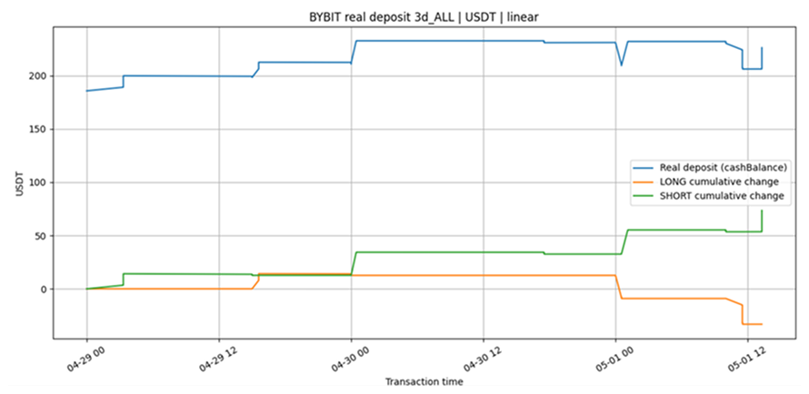
Figure 1. Simulation results.
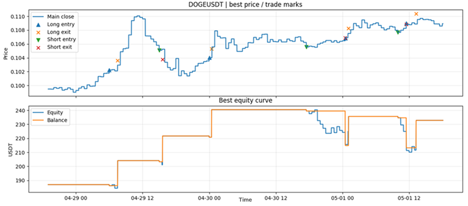
Figure 2. Live trading results from the automatic bot.
As can be seen, the profit trajectories are broadly close in overall tendency. But, and this is an important "but", the number of positions, as well as their character, can differ substantively.
In our case, this difference, as practical experience shows, gradually evens out on extended time intervals in terms of profit and in terms of the ratios of trade counts:
long+ / long-;
short+ / short-;
profit-take / signal close / stop-loss.
But it is not required to even out in terms of the precise times of position entries and trade closures.
This is a fundamentally important point. A live bot should not always be expected to match simulation "trade for trade" on a short window. On a small interval, such agreement may be more a matter of fortune than an obligatory property of a correct model.
The more appropriate level at which to compare is aggregate statistics:
trades per day;
long and short share;
win rate for long and short;
mean PnL per trade;
profit factor;
commissions as a share of gross profit;
maximum drawdown;
distribution of close reasons;
convergence of results across different exchanges.
If these metrics converge over a large number of trades, the simulation model can be considered sufficiently close to reality, even if individual entries and exits do not coincide perfectly.
Synchronisation: Important, But Not Always Necessary
Theoretically, one can attempt to synchronise the simulation and the live bot.
This would require knowledge of the state of the live bot at the moment the window begins:
whether there is an open position;
at what price it was opened;
the volume of the position;
whether a waiting period is active;
which active orders exist;
the current balance;
the last signal received;
the time of the most recently processed candle.
The simulation can then be launched not "from scratch" but from the real state of the bot.
In practice this is far from trivial. Moreover, it is not always necessary.
If the goal is not to demonstrate agreement on a specific trade but to evaluate the quality of the algorithm, then on a sufficiently long interval the influence of the initial state should diminish. As the number of trades grows, the initial phase gradually dissolves into the statistics.
It is for this reason that, in analysing a bot, it is important to correlate profit not only with calendar time but with the number of trades. If a bot opens 8 to 9 positions over three days on a single exchange and simultaneously runs on two exchanges, around 160 to 180 trades can accumulate over a month. This is a substantially more informative sample than a single short three-day fragment.
Naturally, two exchanges trading the same pair do not provide fully independent observations: the underlying market is the same, and price movements are strongly correlated. They remain useful nonetheless, because they allow comparison of algorithm stability, the influence of execution quality, commissions, latency, data accuracy, and the divergence between reality and simulation.
Practical Implications
The aspects discussed above effectively reduce to the following thesis:
“A trading bot should produce stable profitability across any sufficiently long fragment of the market.”
But the view through ergodicity adds an important nuance.
It is insufficient to say "the bot earned X over the period". One must ask:
how many trades were executed;
what was the mean profit per trade;
what was the dispersion of the result;
what share went to commissions;
how were long and short distributed;
how sensitive was the result to the initial point;
do simulation and live trading results converge over extended statistics;
does the result persist after a change in market regime.
In practice, particularly in tournaments and championships of automated trading, the factor of the initial point can play a substantial role. A fortunate market entry, and the entire trading history over a short interval may appear highly promising.
The weak repeatability of championship winners' results year over year, where it has been documented by the statistics of a given championship, can serve as a further illustration of these claims. The MetaQuotes Automated Trading Championships from 2006 to 2012 and the World Cup Trading Championships from 1983 to the present have produced a substantial record of this pattern, which we examined in our previous review [3].
Conclusion
A trading bot is not merely a signal formula.
In live trading, it becomes a system with memory: with state, with an execution phase, with open or recently closed positions, with latency, with commissions, with slippage, and with the constraints of exchange infrastructure.
This is why a short backtest can mislead. It may be not simply a "small sample" but a sample distorted by the initial state of the trading automaton.
On long intervals with a sufficient number of trades, this influence should diminish. But if the strategy is marginally profitable and the number of trades is small, the influence of the initial segment may be comparable in magnitude to the entire visible profit for the period.
For this reason, in analysing trading bots it is important to look not only at profit but at the statistical structure of the result: trade count, mean PnL, dispersion, long and short balance, reasons for closure, commissions, drawdowns, and stability across different time fragments.
In our view, considering automated trading through the lens of ergodicity does not displace the classical approaches to strategy analysis. But it adds an important practical nuance: a live bot does not exist in an idealised model. It exists in time. And it enters each new period not with a clean slate, but with its own history.
And history, as we know, sometimes decides a great deal.
This material is analytical and technical in nature and does not constitute investment advice.
References
[1] Barker, W. and Pomeranets, A. (2011). "The Growth of High-Frequency Trading: Implications for Financial Stability." Bank of Canada Financial System Review, June 2011, pp. 47-52. https://www.bankofcanada.ca/wp-content/uploads/2011/12/fsr-0611-barker.pdf
[2] U.S. Securities and Exchange Commission and U.S. Commodity Futures Trading Commission (2010). "Findings Regarding the Market Events of May 6, 2010." Report of the Staffs of the CFTC and SEC to the Joint Advisory Committee on Emerging Regulatory Issues, September 30, 2010. https://www.sec.gov/news/studies/2010/marketevents-report.pdf
[3] Solovyov, V. (2026). "Do Neural Networks Actually Work for Financial Markets?" Teresius AI. https://teresius-ai.com/news/do-neural-networks-actually-work-for-financial-markets
[4] Bybit. "Rate Limit." V5 API Documentation. https://bybit-exchange.github.io/docs/v5/rate-limit
[5] Poloniex. "Public Channels." Spot WebSocket API Documentation. https://api-docs.poloniex.com/spot/websocket/
[6] Binance. "Kline/Candlestick Data." Spot API Documentation. https://developers.binance.com/docs/binance-spot-api-docs/rest-api/market-data-endpoints
[7] "Slippage (finance)." Wikipedia. https://en.wikipedia.org/wiki/Slippage_(finance)
[8] Peters, O. (2019). "The Ergodicity Problem in Economics." Nature Physics 15, 1216-1221. https://www.nature.com/articles/s41567-019-0732-0
[9] Bailey, D. H. and López de Prado, M. (2014). "The Deflated Sharpe Ratio: Correcting for Selection Bias, Backtest Overfitting, and Non-Normality." Journal of Portfolio Management 40(5), 94-107. For an accessible summary of the framework, see Bailey, D. H. and López de Prado, M. (2021). "How 'backtest overfitting' in finance leads to false discoveries." Significance, Royal Statistical Society. https://rss.onlinelibrary.wiley.com/doi/10.1111/1740-9713.01588