Multifractals and Financial Markets: On the Possibility of Universal Patterns
Fractal Geometry: From Nature to Markets
In 1982, Benoît Mandelbrot published The Fractal Geometry of Nature, a landmark work that formalized the concept of fractal structures and gave mathematicians and scientists a rigorous vocabulary for describing self-similarity across scales. The central insight is deceptively simple: many natural systems — coastlines, clouds, trees — look statistically similar whether you observe them from a kilometer away or a meter away. This property, called scale invariance, turns out to be surprisingly common.
What most introductions skip over is that Mandelbrot had been applying this thinking to financial markets nearly two decades earlier. His 1963 paper on cotton price variation showed that price fluctuations follow heavy-tailed, non-Gaussian distributions that look similar across different time scales – an observation that contradicted the smooth, bell-curve assumptions underlying classical finance theory of the era. The 1982 book consolidated and generalized these ideas into a coherent geometric framework.
By the late 1980s, practical implementations began to emerge. Michael Barnsley introduced Iterated Function Systems (IFS) in Fractals Everywhere (1988), enabling the computational modeling of complex fractal structures. A decade later, multiscale wavelet methods became foundational in signal processing and image compression – JPEG2000 uses wavelet transforms as its mathematical backbone. These were the first signs that fractal thinking could produce working engineering tools, not just beautiful pictures.
What Is Multifractality, and Why Does It Matter for Finance?
A standard fractal is described by a single scaling exponent – one number characterizes how the structure behaves at every scale. Multifractals generalize this: they require a spectrum of scaling exponents, because different parts of the system scale differently. Think of it this way: during a quiet trading week, price moves are small and smooth; during a crash, they are sudden and violent. A single exponent cannot describe both regimes simultaneously. A multifractal model can.
Formally, the key tool here is the Hurst exponent H, which measures persistence in a time series. H = 0.5 corresponds to a pure random walk; H > 0.5 means trends tend to persist; H < 0.5 means reversals are more likely. In a multifractal system, H is not a fixed constant – it varies locally over time, which is exactly what we observe in real markets: volatility clusters, quiet periods are interrupted by turbulence, and the character of price movement shifts across different time horizons.
This raises a concrete and testable question: can multifractal structures be reliably identified in financial data using formal mathematical methods?
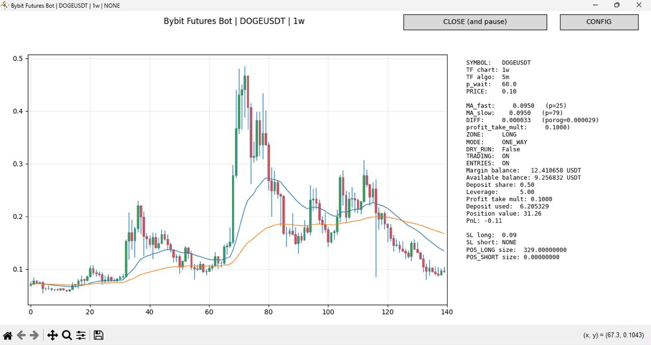
Weekly candlestick chart (1w timeframe). The highlighted segment spanning candles 80–120 on the x-axis shows a distinct price formation — a peak, decline, and partial recovery — with both moving averages (fast: blue, p=25; slow: orange, p=79) reflecting the underlying momentum structure at this scale.
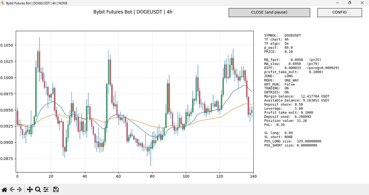
Four-hour candlestick chart (4h timeframe) of the same asset. The highlighted segment spanning candles 80–130 on the x-axis displays a geometrically similar pattern: the same rounded consolidation, directional shift, and recovery shape — but compressed into a much shorter clock-time window.
The visual similarity between the two formations, observed across timeframes that differ by a factor of 42, illustrates a core property of multifractal systems: structural self-similarity across scales. This is not coincidence — it is the empirical signature that multifractal analysis is designed to detect and quantify.
What the Research Actually Shows
Several major research programs have tackled this question, each from a different angle.
Mandelbrot, Fisher, and Calvet (1997) introduced the Multifractal Model of Asset Returns (MMAR) in a Cowles Foundation working paper. The MMAR models price changes by subordinating a Brownian motion to a multifractal time-deformation process – in plain terms, it separates "what happens" from "when it happens," allowing the model to capture both the heavy tails and the long memory of volatility observed in real markets. The MMAR was the first model to achieve scale consistency: the same scaling law holds whether you sample prices by the minute or by the week.
Mantegna and Stanley (1999) approached markets from the perspective of statistical physics in Introduction to Econophysics: Correlations and Complexity in Finance (Cambridge University Press). Their contribution was methodological: they showed that tools developed to study physical systems near critical points – power laws, scaling, universality – apply with surprising precision to financial time series. This opened a productive line of cross-disciplinary research.
Bacry, Delour, and Muzy (2001) introduced the Multifractal Random Walk (MRW), a mathematically elegant process with exact multifractal properties and stationary increments. It is the first continuous stochastic process that simultaneously satisfies these two properties, making it a more tractable alternative to the cascade-based MMAR for both simulation and estimation. For a deeper look at how these methods are applied in practice, see our earlier analysis of forecasting financial markets using multifractal neural networks.
Kantelhardt et al. (2002) contributed the practical measurement toolkit. Their paper, "Multifractal detrended fluctuation analysis of nonstationary time series" (Physica A, 316, 87–114), introduced MF-DFA – a method that detects and quantifies multifractal structure in data without requiring stationarity. MF-DFA works by computing how the root-mean-square of local fluctuations scales with the window size, across a range of moment orders. It has since become one of the most widely used empirical tools in quantitative finance research.
Despite this substantial body of work, a critical practical gap remains: demonstrating that multifractal structure exists in financial data is not the same as demonstrating that it can be extracted and exploited reliably in a real trading system operating under live market conditions.
Where Neural Networks Enter
Modern deep learning provides a natural complement to multifractal theory. Neural networks are universal function approximators – given sufficient data and architecture, they can learn complex, nonlinear, multi-scale dependencies without requiring the researcher to specify the functional form in advance. This is valuable precisely because which relies on multifractal pattern analysis as one of its two core methods alongside LSTM neural networks and sensitive to the choice of parameters.
In practice, a neural network trained on price history can learn representations that implicitly reflect multifractal structure, without explicitly computing scaling exponents. This is both the strength and the limitation of the approach: the model may generalize well empirically, but it provides limited interpretability about why it works when it does.
The Universality Hypothesis
This leads to a deeper and more provocative question: can a single model describe multiple financial instruments simultaneously?
Empirical observation suggests that many market patterns are structurally similar across assets. The volatility smile in options markets, the heavy-tailed distribution of daily returns, the long-memory property of absolute returns – these appear in equity indices, foreign exchange pairs, and cryptocurrency markets alike. The differences are often quantitative (different scaling exponents, different volatility levels) rather than qualitative (different mathematical structure).
If this is true, it implies a form of universality – the same mathematical laws govern very different markets, much as the same physical laws govern very different fluids. This is not metaphor: in statistical physics, universality classes are rigorously defined, and some researchers have argued that financial markets may belong to identifiable classes.
The practical implication is significant. If universality holds, then normalization – transforming different assets into a common representation by removing asset-specific scale – allows a single model to be trained across instruments simultaneously. Volatility scaling (dividing returns by a rolling volatility estimate) and local mean normalization are the most common techniques. The result is a shared parameter space that does not depend on whether the underlying asset is EUR/USD, Bitcoin, or a commodity future.
Teresius Forecast: A Practical Implementation
The Teresius Forecast system, available via@teresius_ai_bot on Telegram, is a working example of this universality approach. A single trained model generates price range predictions – high, low, close, and estimated volatility – across multiple cryptocurrency pairs (BTCUSDT, ETHUSDT, ADAUSDT, and others) and across multiple timeframes (30 min, 1h, 2h, 4h, 1 week), without instrument-specific retraining.
This is architecturally meaningful: it suggests the model has learned representations general enough to transfer across assets, which is consistent with the universality hypothesis described above.
One important caveat the Teresius team explicitly acknowledges: predicting the likely price range of an asset is not the same as generating profitable trades. Execution costs, slippage, position sizing, and risk management all determine whether a statistically useful forecast translates into positive returns. Forecasting accuracy and trading profitability are related but distinct problems.
How Pieoneers Builds Systems Like This: AI-Assisted Development in Practice
Building a production forecasting system – one that ingests live exchange data, runs inference in real time, and delivers results through a conversational interface – involves a significant engineering surface. At Pieoneers Software Inc., the team behind the Teresius Forecast infrastructure, AI coding tools are now a central part of how that surface gets covered.
Specifically, the development workflow for Teresius leverages Claude Code (Anthropic's agentic command-line coding assistant) and OpenAI Codex for different aspects of the build. Claude Code is used for architecture-level reasoning tasks: reviewing system design, generating boilerplate for data pipelines, writing and refactoring the model evaluation and backtesting code, and producing documentation that stays current with the codebase. Codex is used for faster, context-specific completions within the IDE during active development sessions.
The practical effect is a meaningful compression of the time between research prototype and production deployment. Code that would previously require a senior engineer to write from scratch – data normalization pipelines, API integrations with Binance Futures, Telegram bot infrastructure, model serving logic – can be scaffolded by AI tools and then reviewed, tested, and refined by the engineering team. The engineers remain responsible for correctness, performance, and architectural decisions; the AI tools accelerate the execution.
This reflects a broader approach at Pieoneers: the company has been an early and deliberate adopter of AI tooling across its client work, not as a replacement for senior engineering judgment but as a force multiplier for it. The Teresius project is a direct demonstration of that philosophy — a research-grade forecasting system built and maintained by a small, senior team, with AI coding tools closing the gap between ambition and delivery speed.
For fintech teams, academic research groups, or startups exploring similar systems, Pieoneers brings both the technical capability and the operational experience of having built and deployed AI-assisted development workflows at production scale.
Conclusion
Multifractal theory offers a rigorous conceptual framework for financial markets – one grounded in decades of mathematical research and increasingly supported by empirical evidence. The core ideas (scale invariance, heterogeneous scaling exponents, volatility clustering, universality across instruments) are well-established in the academic literature. The tools for measuring multifractal structure in data (MF-DFA, MRW models, MMAR estimation) are mature.
What remains open is the engineering challenge: reliably extracting and operationalizing these structures in live trading environments, at scale, across a wide range of market conditions. Neural networks represent the most promising current path for closing that gap – not because they solve the theoretical problem, but because they sidestep it, learning empirically what multifractal theory predicts analytically.
The Teresius Forecast system is one rigorous attempt to bridge that distance. Whether the universality hypothesis holds broadly enough to sustain the approach across asset classes and market regimes remains an open and productive research question.
References
Mandelbrot, B.B. (1982). The Fractal Geometry of Nature. W.H. Freeman.
Barnsley, M. (1988). Fractals Everywhere. Academic Press.
Mandelbrot, B.B., Fisher, A.J., and Calvet, L.E. (1997). "A Multifractal Model of Asset Returns." Cowles Foundation Discussion Paper No. 1164, Yale University.
Mantegna, R.N. and Stanley, H.E. (1999). Introduction to Econophysics: Correlations and Complexity in Finance. Cambridge University Press.
Bacry, E., Delour, J., and Muzy, J.F. (2001). "Modelling financial time series using multifractal random walks." Physica A, 299(1), 84–92.
Kantelhardt, J.W., Zschiegner, S.A., Koscielny-Bunde, E., Havlin, S., Bunde, A., and Stanley, H.E. (2002). "Multifractal detrended fluctuation analysis of nonstationary time series." Physica A, 316, 87–114.